Autodesk Inventor Tutorial for Beginners: 12 Steps to Success

In this Autodesk Inventor tutorial, you’ll learn the basics of creating and editing 3D models. Read on to see how it's done!
Autodesk Inventor is ideal software if you’re looking to design objects for 3D printing. It’s also an excellent tool for engineers’ assemblies made from multiple parts, as you can import, edit, and export common mesh files like STL or OBJ. If you’re used to other CAD software, Inventor’s user interface is comparable with SolidWorks and SolidEdge.
In this article, we’ll walk you through an Autodesk Inventor tutorial that will teach you the basics of the software. The best part? You don’t need any previous knowledge. Following the step-by-step guide, you’ll be able to build a 3D model of a mug with a handle from scratch. You can even fill it up with a beverage!
But first, let’s briefly cover the basics of technical drawing before pivoting to getting started in the software and diving into the tutorial.

Technical Drawing 101
Autodesk Inventor is parametric design software that relies on relationships, constraints, and dimensioning to characterize the geometry of a model. If the relationships and constraints are correctly set, updating a dimension or feature will automatically update and redraw the entire part geometry. This is different from Autodesk’s AutoCAD, which contains parametric features but is mainly a layer-based software. A change in a property of a drawing layer will automatically change all the objects related to that single layer.
Apart from certain exceptions (i.e. Freeform and Sculpt modeling), the parametric design modeling process consists of drawing a sketch, then building a volume from it. You can perform most of these tasks with commands in the Create panel in Inventor. For example, extruding a sketch, adding width to its area, or revolving its area in space.
To completely understand how this process works, we first have to cover some technical drawing principles, which are the conceptual base of parametric software. The main concern in technical drawing is to represent unambiguously a 3D object in two dimensions, that is, in a plane. Therefore, the two-dimensional representation of the object has to be as precise as possible.

In descriptive geometry, there are various types of image projection. The one that offers the most precise views, considering a lack of deformation, is the parallel orthogonal projection. It considers that the observer of the object is so distant from the plane and the object that the visual rays emerging from the observer’s eyes reach every point of the object and the plane as parallel lines. The parallel projection is orthogonal when the visual rays reach the plane at a 90° angle. The effect is that the projection has the same size as the object and doesn’t present deformation.
This differs from the perspective projection, which assumes that the observer is placed at a finite distance from the plane and object. Here, the visual rays are conic, diverging from the observer’s eyes and reaching the plane. It’s what happens when we turn off the lights and make animal shadows on the wall with our hands using a flashlight. The shadow (projection) is bigger than our hand because the light source is near the object, so the light rays form a cone. The effect is that the projection resembles the visualization of an object with human eyes, with deformation.
On the other hand, taking the analogy of someone playing with shadows, the farther the flashlight is from the hands and the wall, the more the light rays will tend to be parallel and the more the projection on the wall will be similar to our hand’s contour and size, without deformation, resembling an orthographic projection. That’s the one used in Inventor to display models.
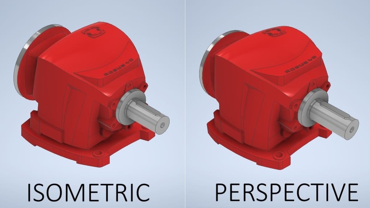
Depending on the orientation of the object relative to the observer’s eye, orthographic view and axonometric projections can originate in the parallel orthographic projection. In Inventor, you see orthographic view projections in the Graphics Display when you click on a face of the View Cube (more on this later). Axonometric projections are the other visualizations of your model when you rotate it. The most used axonometric view is the isometric projection, which is the one you see when clicking on one of the View Cube corners.
This information may seem a little abstract, but it’s useful. These concepts are present when visualizing a model in the Graphics Display, and they’re also the basis of all modeling processes in parametric software. It’s required, for most cases, that you first choose a face of the object you’ll model, then draw its contours in the Sketch environment.
So, the first thing you’ll draw is one of the orthographic projection views of your object. After that, you’ll give volume to the sketch by using one or more commands on the 3D Model ribbon tab. These steps will become clearer in our tutorial.
Getting Started
First up, be aware that Autodesk Inventor requires specific hardware capabilities. The software is mainly available for Windows PCs. To access the software on Mac computers, additional steps must be taken. The system requirements for Windows can be easily accessed on the Autodesk website for the latest and previous versions.
Autodesk Inventor is a paid software with different subscription plans. However, it’s also available as a 30-day free trial if it’s the first time that you’re downloading it with your Autodesk account. If you don’t have an Autodesk account, you’ll need to create one and register on the website.
After your trial period, you’ll need to subscribe to a plan to continue using the software. If you’re a student or teacher, you can sign up in the Educational Community for free software licensing for one year. After the first year, it’s possible to renew the licensing through an educational verification.
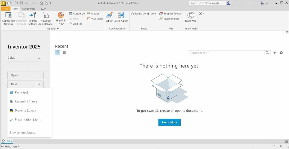
After downloading the software, follow the installation wizard steps until you’re able to open it. When opening Inventor for the first time, you’ll see the Home window, as shown in the previous image. Every drawing in Inventor is opened based on a template, which is an empty drawing file with some preset configurations of measurement units and the drawing standard.
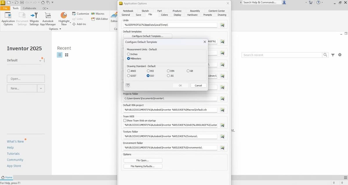
It’s important to be aware of the measurement units you’ll be drawing before starting. To change them, follow these steps:
- Open the File menu and click on the Options button at the bottom. This will open the Application Options window.
- Select the button called “Configure Default Template…” in the File tab.
- Configure the measurement units and the standard as you wish in the window that opens. We’ll use millimeters for the units and the ISO standard for this tutorial.
- Click OK to confirm.
UI Overview
There are two ways of opening the main drawing environment in Autodesk Inventor. The first is by clicking on “New…” on the left panel of the homescreen and the second, by clicking the drop-down arrow just next to it, then selecting “Part” from among the options.
If you click on the “New…” button, you’ll be able to choose the template to build your drawing on. If you open the panel and click on “Part”, it will automatically open the environment drawing considering the default template, which we previously set.
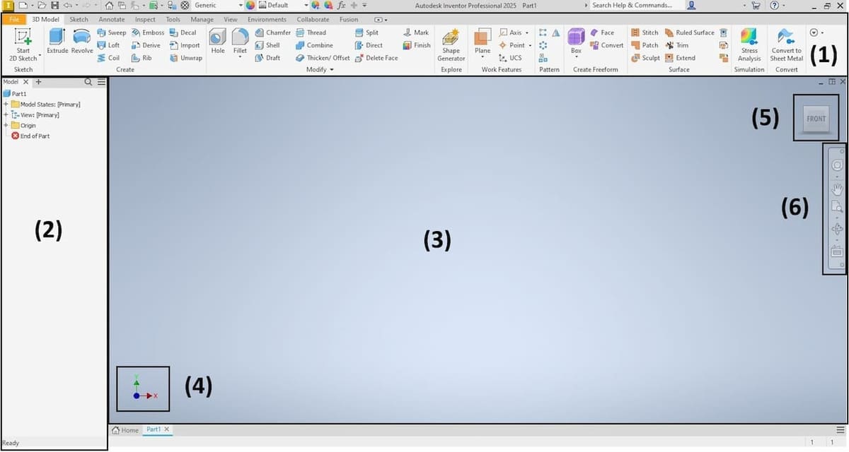
The drawing environment is called the Application Window and contains the following tools and features:
- Ribbon tabs and commands (1)
- Model Browser on the left (2)
- The Graphics Display screen, or viewport, which is the most important screen in the Application Window (3)
- The Cartesian Coordinate System on the bottom-left corner (4)
- The View Cube in the top-right corner (5)
- The Navigation bar immediately below the View Cube (6)
Visualizing Objects
Visualizing your model is an important part of the design process. Within Inventor, there are a couple of tools that can help you with the visualization process. Both Coordinate System and View Cube will help you to orient the visualization of your model on the Graphics Display screen, whether by clicking on a coordinate axis or a face, edge, or corner of the View Cube.
The View Cube shows the model from an axonometric perspective, among them the orthographic views and isometric views. If you hover over the cube, you can see a little house that will center the model on an isometric view. You can change the home view by first switching to your preferred point of view. Then, right-click the home symbol > Set Current View as Home > Fit to View.
The default projection system of Inventor’s Graphics Display is orthographic. However, it’s possible to change it to the perspective projection by right-clicking the home symbol in the View Cube > Perspective.
Throughout your design work in Inventor, you’ll use your mouse to control the visualization of your Part, so let’s learn how to do this.
- Click and hold the scroll wheel in the middle of the mouse to move the visualization in a plane (i.e. “to pan” the view).
- Hold Shift on the keyboard and hold the scroll wheel simultaneously to rotate the view 360° (i.e. “to orbit” the view).
- Scroll with the mouse wheel to zoom the view in or out toward the cursor’s position.
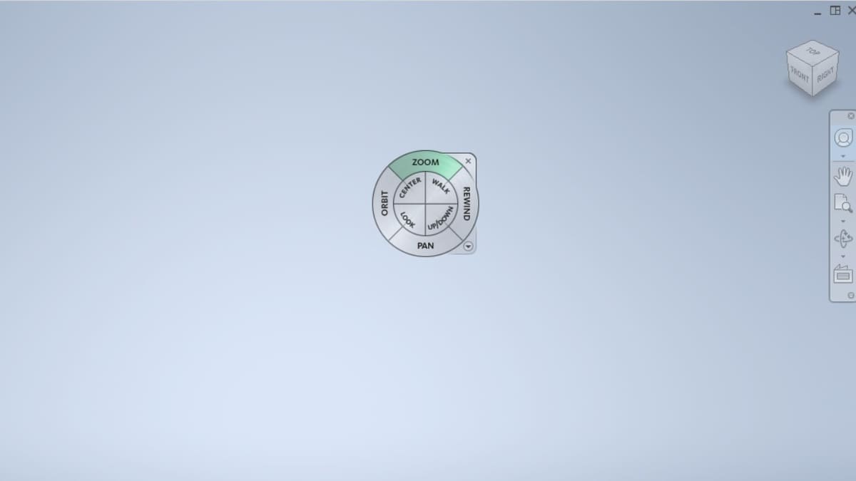
If you’re working on your laptop and don’t have access to a mouse, you can enable the Full Navigation Wheel in the Navigation Bar. That way you can access each movement tool mentioned previously (pan, orbit, and zoom) separately.
Tutorial
Now that we’ve covered the basics, we’re ready to start our Autodesk Inventor tutorial, in which we’ll build a simple model of a mug with a handle filled with a beverage.
Part I: Parametric Sketching
In this first part, we’ll design the main sketch for our mug. As mentioned in the UI Overview section, when the Application Window is opened, we can enter the sketching environment with the 3D Model ribbon tab, by clicking on the feature “Start 2D Sketch”. When clicking on it, the Sketch ribbon tab opens.
For Part 1 of our tutorial, we’ll use the following commands from the panels of the Sketch ribbon tab:
- Create: Line, Arc, Fillet
- Constrain: Dimension and the constraints Coincident, Collinear, Horizontal, Vertical, Tangent, and Symmetric
- Format: Centerline
The Create panel contains the commands to draw the main elements in the sketch, such as Lines, Arcs, Rectangles, and Circles, among many others. The Constrain panel commands will be used to add relationships between the drawing elements, as will be detailed below. The Format panel includes commands that change drawing element features, like turning a line into a centerline or a construction line.
Step 1: Choose a Plane
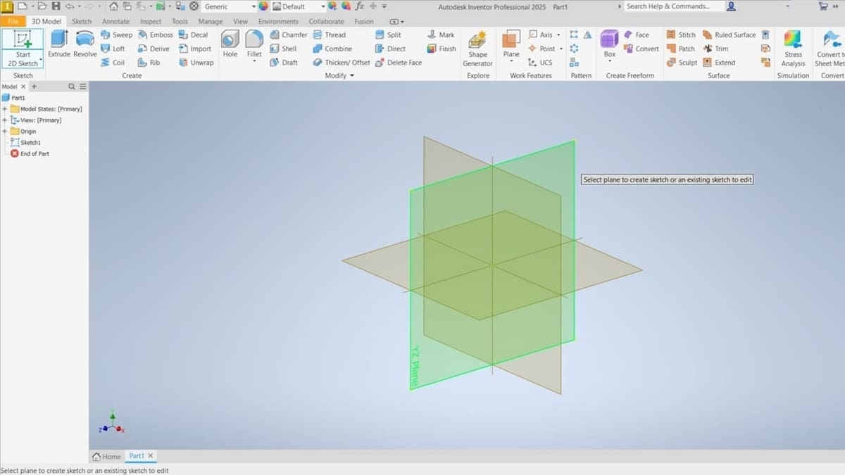
When entering the sketching environment, it will show the three Cartesian planes intercepting the origin of the Cartesian coordinates. In this step, we should choose the plane upon which we will draw the orthographic contours of our model. Here is a stalemate: Which plane to choose?
Let’s think about playing with a mug’s shadows: If we put a mug in front of a distant flashlight, its contours would be clear on the wall without deformation, and the dimensions of the projection would be quite close to the dimensions of the mug. We want to find the plane of the wall. Thinking of the contours of a mug (not considering the handle), we should be able to identify that it’s symmetrical – that is, one side of the contour is exactly like the other side, and there is an imagined vertical centerline dividing both sides.
The key to choosing the right plane to start sketching is to imagine which of the planes would be the wall showing the mug’s contour. Looking at the Cartesian planes and the origin in Inventor, we could imagine that the vertical centerline is the Y-axis (the green arrow in the origin). Therefore, the wall plane could be the YZ-plane or the XY-plane. Let’s choose the YZ-plane, noting that both will produce the same view. So, a good sketch would be the mug contour (i.e. the orthographic projection) placed in YZ-plane.
If we had a real object, the preparation step before drawing would include measuring its dimensions. One good design tip for beginners starting 3D modeling is to choose some simple objects you have in your home to replicate in the software. Just copying other people’s models will prevent you from tinkering with the task and becoming independent.
Step 2: Add Reference Lines
We can now start sketching a rough draft based on the general geometry of the chosen orthographic view of the object. We’ll use the some of the Create panel commands, including Line, Arc, and Fillet.
The very first thing we’ll do is to draw two lines, which will be our Y and Z references. To create a line, click on the Line command. You’ll be requested to set the first point, which you can do by left-clicking at some point in the plane, then dragging the mouse without clicking to set the length of the line. Finally, you’ll be requested to select the endpoint of the line. You can left-click again to set it at some point of the plane. It’s possible to see what the command is requesting in the Status bar, the bar located beneath the Model Browser and Graphics Display screen.
So, let’s start creating the reference lines for our mug:
- Click in the origin and drag the mouse to nearly 70 mm in length to make the mug 70 mm in height.
- Click to set the endpoint aligned to the first point (i.e. 0 degrees). When it’s finished, the line should turn black. This line is our vertical reference, being an important construction element in the sketch.
- Select this line and click on the Centerline command in the Format panel.
- Create the horizontal construction line. Here, the length of the line isn’t important, as it’s simply a horizontal reference. So, let’s just create a line with a random length, starting at the origin. Then, make it a Centerline, too.
Throughout the entire process, a dimension input little box with the length of the line and the angle between the line and the Z-axis is shown near the cursor, allowing you to see the real-time length of the line as you drag the mouse in the plane. This way, you’ll be able to select an endpoint approximately 70 mm away from the first point.
Step 3: Draft the Mug
As we’ve seen, the mug contour is symmetrical with a vertical centerline, the Y-axis, defining the halves. Since it is, in fact, a 3D object, the mug has rotational symmetry, and later, we’ll revolve the sketch to obtain the 3D model. So, it’s not necessary to draw the entire contour, but only one half. The contour area enclosed by this half will be revolved 360º in space based on the Y-axis, and a 3D mug will be obtained.
To sketch, we first make a rough draft, not being worried about applying the right dimensions because these will be applied later with the constraints. However, as we draw, some constraints appear naturally, derived from the mug contour geometry. You can think of constraints as rules and limitations that are applied to the drawing elements.
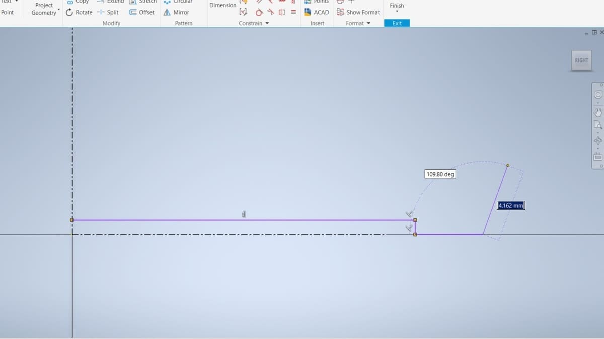
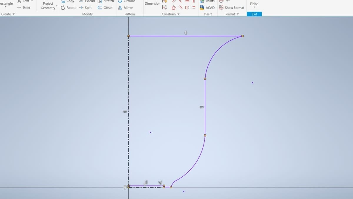
The three lines shown in the image above illustrate the process. Note that because the first and end points of horizontal lines were set aligned, a horizontal symbol appears next to it. This is a horizontal constraint. Whatever modification we set in the sketch, this line will remain horizontal. It can be seen that the symbols of perpendicularity also appear. These ensure that these lines will always be perpendicular.
The next step is to create an arc in the last endpoint drawn. So, it’s necessary to exit the Line command to activate the Arc command. This can be done by pressing ESC on the keyboard or by right-clicking with the mouse anywhere on the Graphics Display. A menu will open with an Ok button, which you’ll want to click.
Arcs
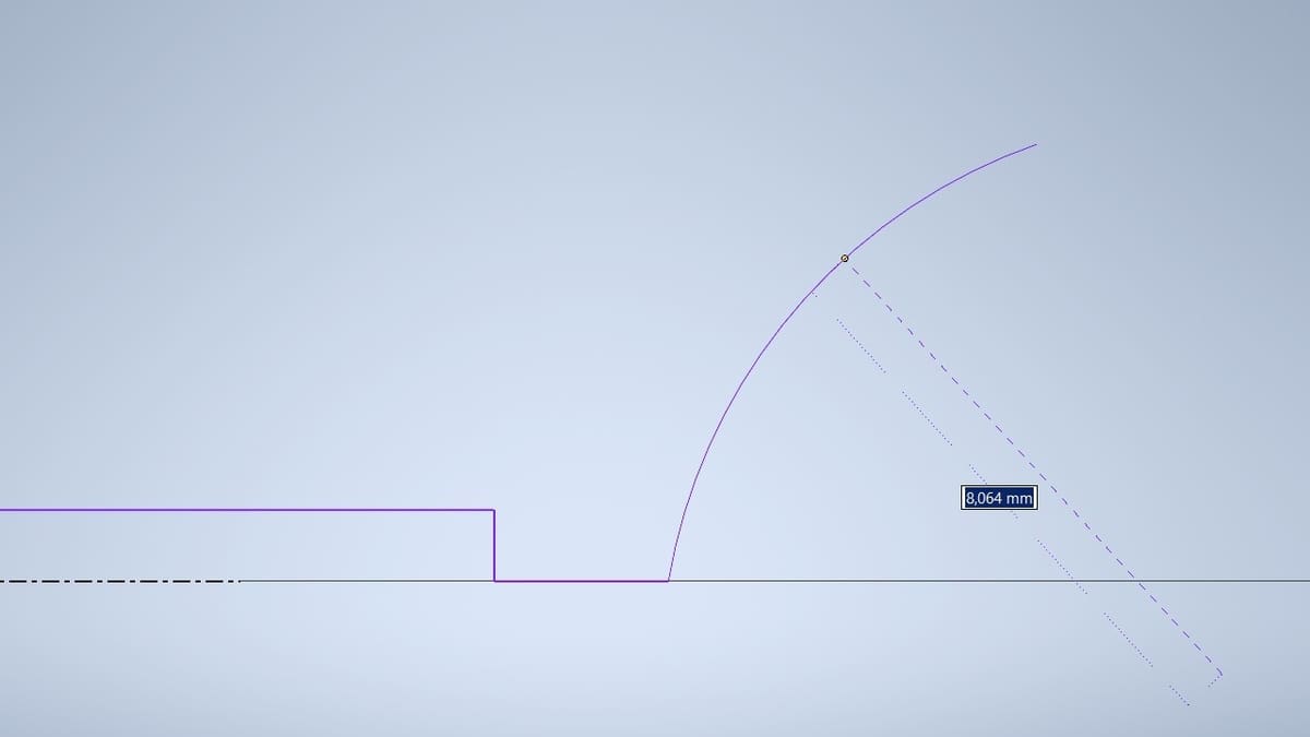
When we click on the Arc button, we’re actually choosing the default Three Point Arc command. Other types of arcs can be found by clicking on the arrow below the Arc button. For building a Three Point Arc, a first point is needed, then the endpoint of the arc, and finally a third point related to the radius of the arc and its curvature – either concave (curves inward) or convex (curves outward). For the first arc, we’ll draw it with approximately 8 mm of radius and make it concave (see image above).
To position the arc’s first point, click on the last drawn line’s endpoint so they’ll be connected. The next point is the arc’s endpoint. Choose a point in the drawing area near to where it would be, considering the overall contour of the mug.
The third point will determine the radius of the arc and whether it will be concave or convex. If you place the mouse on the left of the two points created, you’ll build a convex arc and, placing it on the right, a concave arc. A dimension input little box will always follow the mouse indicating the radius measurement as you move it. This way, you’ll be able to choose a point near the 8-mm radius.
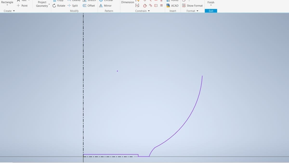
The next arc will be convex and have a radius of 30 mm, so try to stay close to that value, as shown in the image above. The next step is to return to a line, so don’t forget to exit the Arc command.
To finish drafting, do the following:
- Build a vertical line of 20 to 30 mm starting at the endpoint of the last arc drawn. This line represents the diameter of the middle of the mug.
- At the endpoint of this line, draft another concave arc with an approximately 25-mm radius.
The endpoint of this arc will be the point that determines the diameter of the top of the mug. Therefore, it has to be placed at the same height as the vertical reference endpoint, which will determine the mug’s height. To do this, follow these steps:
- Hover over the vertical reference endpoint without clicking on it.
- Immediately after, keeping the cursor aligned in the process, place the cursor at the right of the line that represents the diameter of the middle of the mug, then click to position the arc endpoint. As shown in the image below, this will make the last arc endpoint aligned with the vertical reference line endpoint.
- Draw the third point of the arc to be convex with a radius of 30 mm.
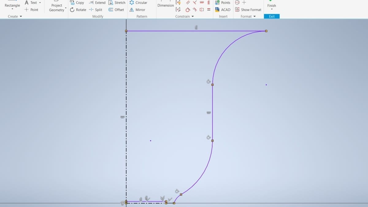
To close the draft contour, create a line between the arc endpoint and the vertical reference endpoint (it will be horizontal if the two points are aligned as done in the last step 2). The final rough draft can be seen in the image below.
The overall geometry of half of your mug is ready. To finish it, it’s necessary to add constraints and dimensions. Let’s move to the fourth step.
Step 4: Apply Constraints
In the image above, you can see the final rough draft with some constraints derived from Step 2. Despite the horizontal and vertical reference lines, all the other lines and arcs are shown in purple. This indicates that these features aren’t fully constrained, meaning they aren’t fully defined in the plane in terms of positioning and dimension. That’s because we haven’t yet applied the dimensions and the totality of constraints.
All the constraints applied until now were put intuitively, considering the overall geometry of half of the contour of the mug. However, some other constraints that aren’t so obvious still need to be placed.
Types of Constraints
When applied, the Coincident Constraints set that two drawing elements are coincident at some point. Throughout the whole draft, there are hidden Coincident Constraints, where we placed the first point of a new element in the endpoint of another. They’re hidden by default to not cause visual clutter on the draft because all the elements are connected, forming a closed area. The Coincident Constraints can be seen by passing the mouse over these points.
Another non-trivial constraint important to our draft is the Collinear Constraint, which makes two elements collinear in the plane. This needs to be applied to the horizontal line that represents the base of the mug and the horizontal reference. This will ensure that the base of the mug will always be aligned with the horizontal reference, which in turn is fixed to the origin. Let’s apply it with the steps:
- Click the Collinear Constraint command in the Constrain panel of the Sketch ribbon tab.
- Select the horizontal reference.
- Select the base of the mug.
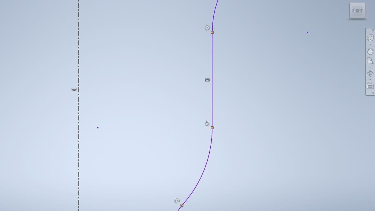
The last non-trivial constraint we need is the Tangent Constraint. It makes drawing elements touch an arc or circle at only one point on the plane, causing the appearance of a smooth transition between them. Therefore, the Tangent Constraint has to be applied between the arcs and all the features that are connected to them whenever a smooth transition between the arc and the element is needed. This can be done as follows:
- Click on the Tangent button in the Constrain panel of the Sketch ribbon tab.
- Select the arc.
- Select the feature connected to it.
- Repeat for all pairs of arcs connected to a feature, except between the arcs and the horizontal lines.
The draft with all constraints applied can be seen in the image below. However, as you can see, the lines are still purple, which means they’re not yet fully constrained. This is because the dimensions of the features have yet to be defined.
Tip
To hide or show all the constraints applied in the sketch, press F8 on the keyboard, or click the button “Hide All Constraints”/”Show All Constraints” at the bottom of the Application Window.
Step 5: Add Dimensions
The next step in order to fully define the sketch features is to add the dimensions. You’ll realize that when fully defined, the feature turns black. Fully constraining a sketch is a way of making your sketch reliable. If you don’t, the software itself will try to find relationships between features. This causes unexpected geometries and creates a 3D model different from what we wanted to build.
To apply the dimensions, we’ll use the Dimension command in the Constrain panel. Then, we’ll click on every drawing element, adding the numerical value of the dimension of the drawing element in the input diameter box near the cursor.
When selecting a line, it will add the value of the length of the line; when selecting an arc, the radius will be configured. It’s also possible to add distances and heights between different features by clicking on their endpoints or a combination of endpoints and features. Using this method, it’s also possible to reference the center of the arcs, shown as points in the sketch.
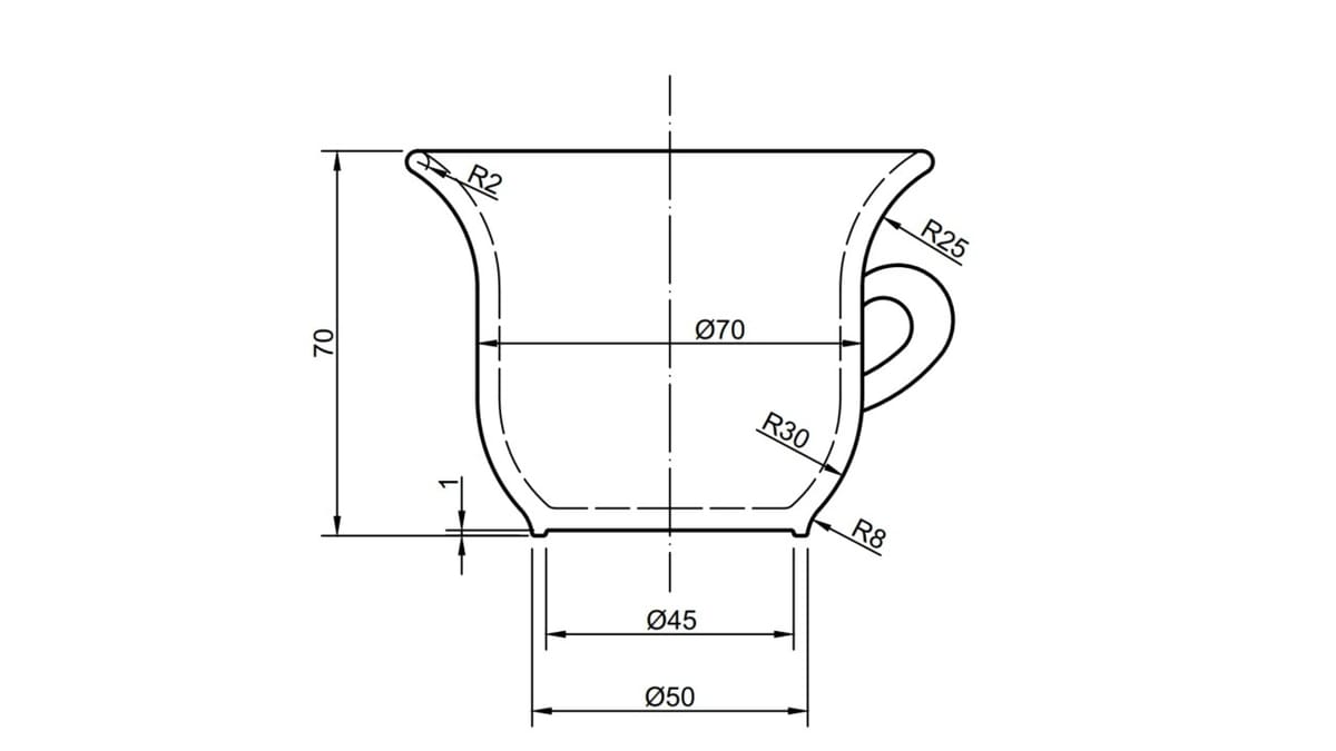
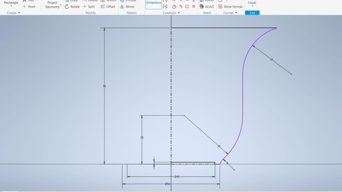
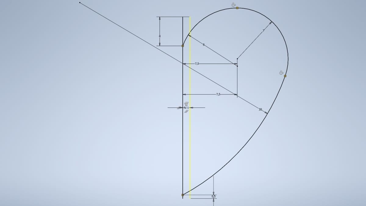
We’ve noted all of the necessary dimensions in the image for Step 2 above. To dimension the features that represent the diameters of the mug, follow these steps:
- Click on the Dimension command in the Constrain panel of the Sketch ribbon tab.
- Select the diameter element (a point of a line that corresponds to the contour of a diameter of the mug).
- Select the vertical reference.
- Add the diameter value in the input diameter box near the cursor. The vertical reference was edited to be a centerline in Step 2, so the software understands that the numerical value that’s entered is a diameter and not a radius.
Repeat the dimensioning process for all drawing elements except for the diameter of the middle of the mug (Ø70 mm in the 2D dimensioned drawing image shown in Step 2) and the diameter of the top of the mug. We’ll need a parametric dimensioning explanation before defining them. The image below shows all the other elements dimensioned in the drawing until now.
Parametric Dimensioning
Every dimension that’s applied in the drawing has an index as “d”, followed by a sequential number. For example, the first dimension applied will be the dimension “d1”, the second will be “d2”, and so on. You can see a dimension’s index by clicking on it directly.
From its index, it’s possible to reference another dimension and create equations. Parametric dimensioning is the act of inputting an index or an equation with indexes instead of a numerical value as the dimension of the feature, making the features interrelated.
Two parametric dimensions can be applied to the mug’s geometry. The first is to relate the diameter of the middle of the mug to its height and the other is to relate the diameter of the top of the mug to the diameter of the middle of the mug. To create a parametric dimension, click on one dimension that was already set when editing the value of another dimension in the input dimension box near the cursor.
Middle Diameter to Height
Let’s start with relating the mug’s middle diameter to its height. We’ll make the diameter the same size as the mug’s height:
- Click on the Dimension button on the Constrain panel of the Sketch ribbon tab.
- Select the vertical line that corresponds to the diameter of the middle of the mug.
- Select the vertical reference centerline. The input dimension box will appear next to the cursor for you to input the diameter of this element.
- Instead of inputting a numerical value, click on the dimension of the centerline (an “fx” symbol will appear near the cursor). The index of the length of the vertical centerline will appear in the input dimension box.
- Press enter on the keyboard.
Top Diameter to Middle Diameter
Now, we’ll relate the diameter of the top of the mug to the diameter of the middle of it (the one that we’ve just configured). We’ll make the diameter of the top 20 mm bigger than the diameter of its middle, using an equation:
- Click on the Dimension button on the Constrain panel of the Sketch ribbon tab.
- Select the endpoint of the horizontal line that corresponds to the diameter of the top of the mug.
- Select the vertical centerline. The input dimension box will appear for you to input the diameter of the top of the mug.
- Instead of inputting a numerical value, click on the dimension of the diameter of the middle of the mug. Its index will appear in the input box, for example, “d12”.
- Write in the input box “+ 20” next to the index value. The final equation in the input diameter box will be, for example, “d12 + 20”.
Step 6: Finalize the Sketch
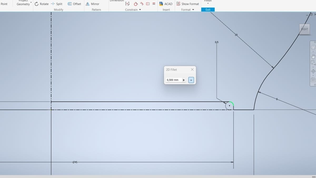
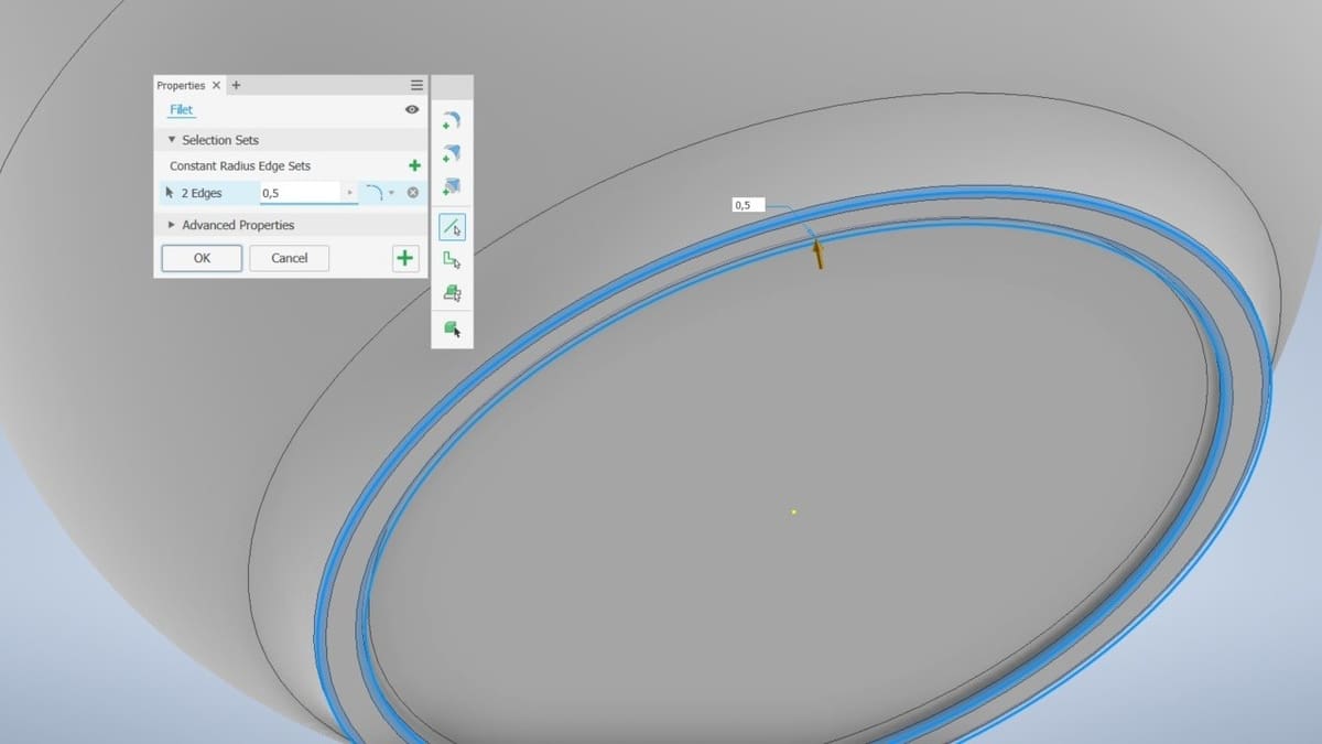
The last addition to be made in the sketch will be modifying a sharp corner with a fillet, which can be found in the Create panel. This feature requires the addition of the right dimensioning value when it’s set, which is the reason why it wasn’t done up until now.
- Click on the Fillet button on the Create panel of the Sketch ribbon tab. The 2D Fillet toolbar will open with an input dimension box.
- Enter the value “0.5 mm”.
- Select the lines that created the sharp edge (i.e., the first two lines drawn in the mug geometry, as shown in the image above).
These were the steps to fully define the mug sketch, and you’ll notice that all the drawing elements are now black. You can leave the Sketch environment by clicking the Finish button in the Sketch tab. We’ll now create a volume from it in the next part of the tutorial.
Part II: 3D Modeling
Part 2 consists of building a volume and effectively 3D modeling the sketch we obtained in Part 1. To do so, we’ll be working in two different ribbon tabs: 3D Model and Sketch.
In the 3D Model ribbon tab, we’ll use these commands in the following panels:
- Create: Revolve, Sweep
- Modify: Shell, Fillet, Thicken/Offset
- Work Features: Point, Plane
- Surface: Patch, Sculpt
The Create panel from the 3D model ribbon is where the commands that create 3D models from 2D sketches are placed. In the Modify panel are commands that modify 3D features created with the Create panel commands. The Work Features panel contains commands that aid with referencing elements in space, such as points, planes, and axes. The Surface panel contains features to construct and modify surfaces.
From the Sketch ribbon tab, the following commands will be used:
- Create: Project Geometry
- Modify: Offset
The Create panel from the Sketch ribbon was extensively used in the last part of the tutorial. Now, we’re adding a command from the Modify panel, which is similar to the same panel from the 3D Model ribbon. However, it’s used in a 2D context to modify sketch elements.
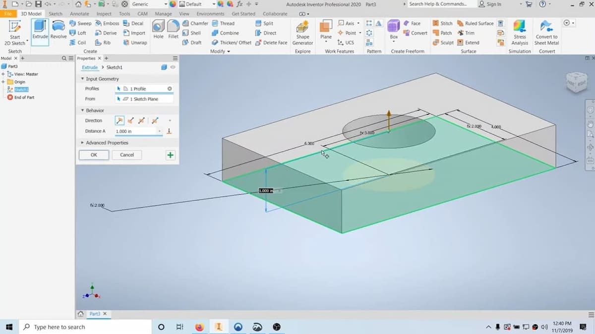
Step 7: Obtain the 3D Design
The main commands used to create a 3D design from a sketch are the Extrude and Revolve commands, located in the Create panel. The Extrude creates a width in the sketch, while the Revolve creates a volume by rotating the sketch in space by a symmetry axis. In the case of the mug, the geometry has a symmetrical axis (the Y-axis), so we’ll use the Revolve command.
- Select the Revolve command. The Revolve Property Panel will appear.
- Click on the fully defined and closed mug sketch to select the required Profile.
- Then, to select the required Axis, click on the rotate axis of the mug (in our case, click on the centerline of our sketch).
- Click Ok on the property panel.
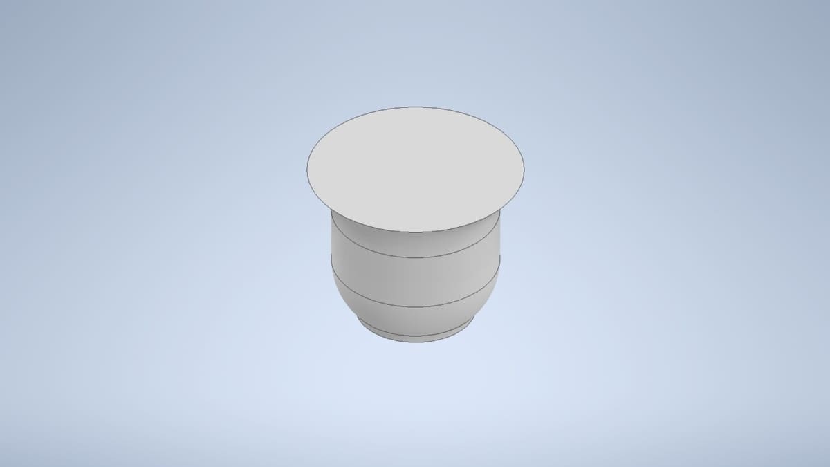
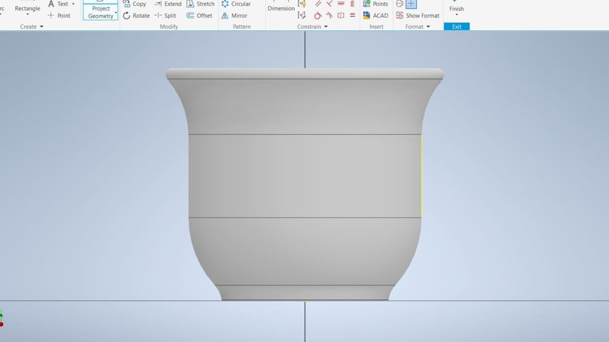
The result is shown in the image above.
Step 8: Edit the Model
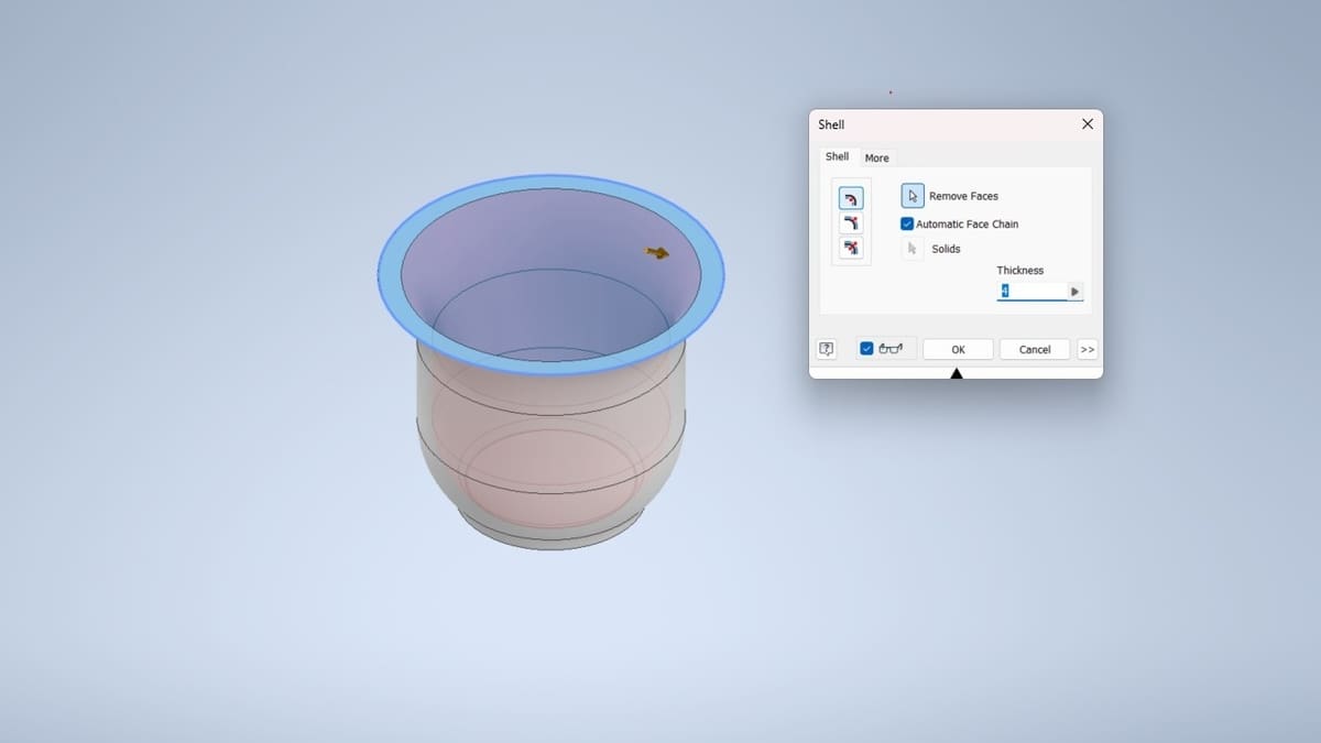
As the previous image suggests, the volume created is fully solid. However, a mug needs to have a hole inside for beverages. To build that hole and maintain it with the same shape as the contour, we’ll use the Shell command in the Modify panel.
- Click on the Shell command. As the model has only one body created by revolving a sketch, the Shell toolbar will open.
- Edit a value of “4 mm” in Thickness input, choosing to remove material from the inside.
- Remove the top surface by clicking on the “Remove Faces” button, then clicking on the top surface.
The Fillet command on the 3D Model tab is the 3D version of the Fillet command from the Sketch tab used in Part 1. It’s another modification in the model that will create smooth edges in some regions.
- Click on the Fillet button on the Modify panel in the 3D Model tab. The Fillet Property Panel will open.
- Set a radius of “2 mm” and set the Smooth G2 type to create smooth edges in some regions.
- Click on both edges of the top surface of the mug to create the mug’s lip.

Now, rotate the model so you can see its bottom, as the image above shows. We’ll apply a fillet in the mug’s foot in this way:
- Click on the Fillet button again.
- Set the radius to 0.5 mm and set the Tangent type.
- Select each edge of the mug’s foot.
By doing this, the mug itself is completed.
Step 9: Sketch the Handle
Now that the mug is almost finished, it’s time to think about the handle design. Here, we’ll repeat the design process we’ve done so far: The 3D model of the handle will be built from a sketch, so an orthographic contour has to be chosen.
The handle has an organic shape and a constant width, so a good 3D model command to obtain this geometry in space would be the Sweep command, located on the Create panel. The Sweep command requires a sketch with a closed region, which will be the cross-section of the handle, and a path orthogonal to it, so it replicates the cross-section throughout the path.
To sketch the path, we’ll use the same YZ-plane, but, as mentioned, the XY-plane would also work. Repeat the actions from Steps 1-3 from Part I to build the path’s sketch using the tools we’ve seen: lines and arc construction, constraints, and dimensioning, mimicking the sketch and the dimensioning from the image above.
- Click the Start a 2D Sketch button in the 3D Model tab. As there’s already a model placed on the Graphics Display, the planes will not appear as the first time.
- To select the YZ-plane, you’ll need to go to the Model Browser and search for it in the Origin folder.
- Click on “YZ Plane”.
Creating the Path
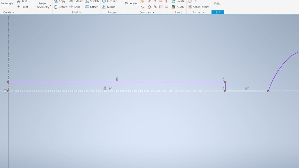
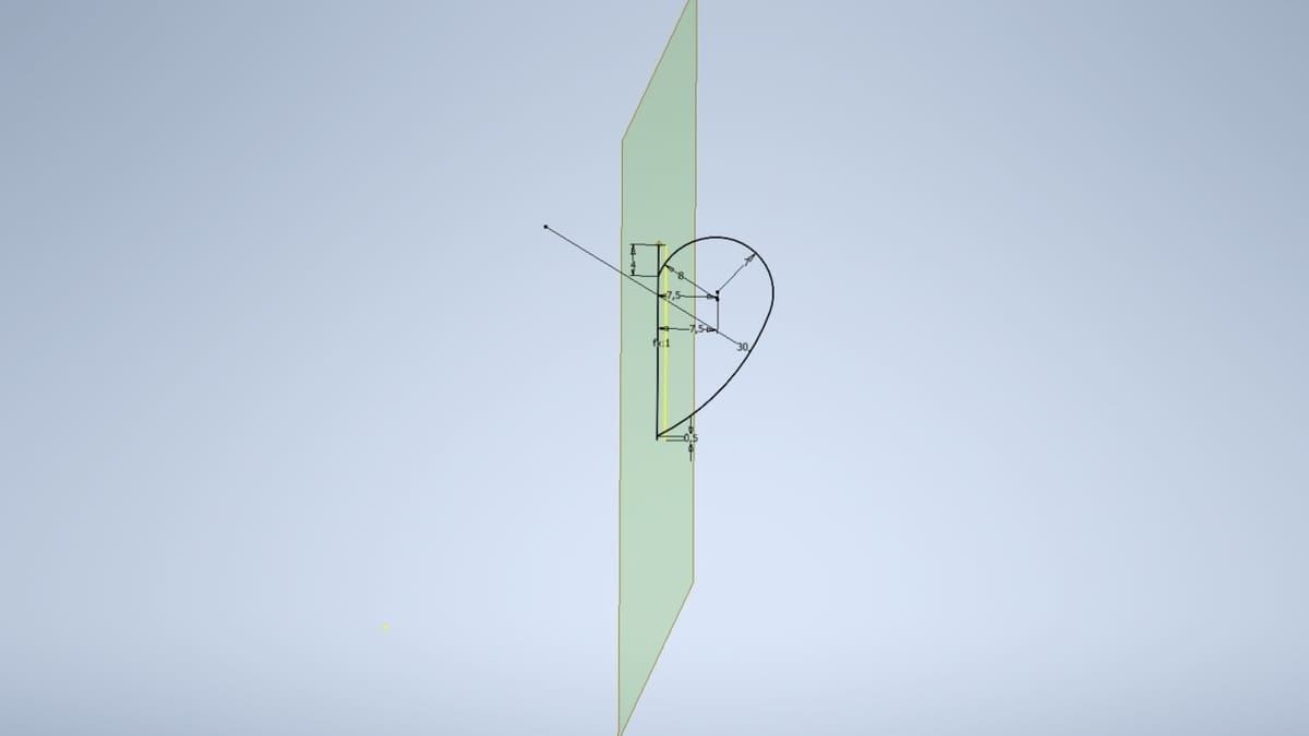
Being inside a new Sketch, as seen before, we first need to create its references. To guarantee the continuity of the model, the path will have to be connected to the contour of the recently created body. To create this type of reference, we’ll use the Project Geometry command. This command will bring the projection of the body’s contour to the current sketching plane, as shown by the yellow line in the image above.
- Select the command Project Geometry on the Sketch ribbon tab.
- Select the contour representing the diameter of the middle of the mug, where the handle would be placed (i.e., the yellow line shown above).
You’ll notice that the black contour will turn and remain yellow. This indicates that the model’s contour turned into a line in this new sketch.
Now, it’s possible to start drafting. Feel free to hide the mug 3D model so it doesn’t cause visual clutter, making it easier to draft. You can change the model’s visibility in the Model Browser by right-clicking on Solid, in the Solid Bodies folder in the browser. Notice that now the only thing you see in the Graphics Display is the origin and the yellow line we’ve just created.
We’ll use the Offset command to obtain a regular fit between the handle and the mug. This makes a copy of a selected feature by some amount of distance. In this case, the path must end inside the mug. So, the offset distance will have to be related to the thickness, and we’ll apply a parametric dimension.
First, we need the index related to the mug thickness:
- Search for the Shell feature in the Model Browser.
- Right-click it to open up the drop-down menu.
- Find the button “Edit Feature”. This will allow you to edit the parameters of the Shell command.
- When the Shell toolbox opens, hover over the Thickness input box without clicking on it. A label next to the cursor will show its index, for example, “d18”.
Now, we can apply the parametric dimension:
- Select the Offset command from the Modify panel of the Sketch tab.
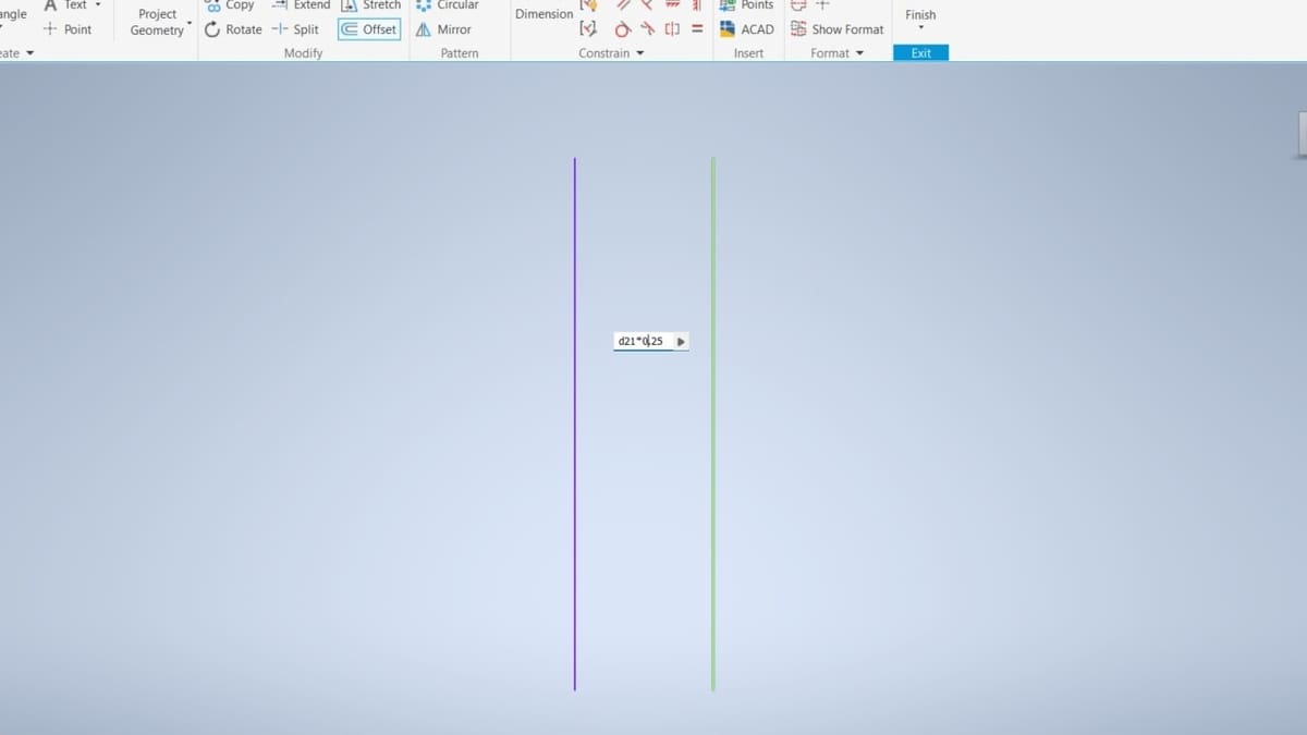
- Select the yellow line that stems from the mug contour. You can drag a copy of this line parallel to the original line as you move the cursor and an input dimension box will appear next to it.
- We want the path of the handle to end inside the mug’s thickness, so put this new line inside the mug’s contour, as the image above shows. This only means we have to put the cursor on the left of the yellow line.
- Set the offset distance to 25% of the mug thickness with an equation: The thickness index we’ve just found multiplied by 0.25 (for example, “d18 * 0.25”).
That way, if the mug thickness changes, the offset distance will change accordingly, since it’s always 25% of the thickness.
The line created by the Offset is now the vertical reference of the handle path. Now, continue to build the sketch with lines, arcs, and the dimensioning shown in the first image of Step 9. After that, you can leave the Sketch by clicking the Finish button in the Sketch tab.
Creating the Handle’s Cross Section
As the path was sketched, it’s only missing the region perpendicular to it (which will be the handle’s cross section). We’ll need this to be able to use the Sweep command. The handle’s cross section must be placed where the path starts. As it starts and finishes in the line created by the Offset, a plane perpendicular to the YZ-plane passing through this line has to be created.
To place a plane in that exact position, you’ll need to first place a point in one of the sketch’s vertical reference endpoints:
- Click on the Point command in the Work Features panel of the 3D Model tab.
- Select one of the endpoints of the line created by the Offset command used before.
Now, we’re able to place the plane:
- Select the command Plane in the Work Features panel of the 3D Model tab.
- Click on the point created above.
- Select the YZ-plane by going to the Model Browser, then searching for “YZ Plane” in the Origin folder.
These steps will build a plane parallel to the YZ-plane, passing through the point created (i.e. passing exactly through the line created by the Offset), as the image above shows.
The last step is to make the handle’s cross section sketch on this new work plane. You’ll use the Project Geometry command one more time to bring a couple of elements from the path onto the new plane, namely the line created by the Offset and the 30-mm arc sketched you created at the end of the Creating the Path subsection. On the new plane, you should see the line which will appear on the plane as a single point.
- Click the Start a 2D Sketch button in the 3D Model tab.
- Select the command Project Geometry on the Sketch ribbon tab.
- Select the line that stemmed from the Offset command from the path’s sketch.
- Select the 30-mm arc from the path’s sketch (you may rotate the view in the Graphics Display to be able to see and click on this arc).
On the new plane, you should now see the line and a single point, which is the endpoint of the 30-mm arc. We’ll use that point to build the handle’s cross section:
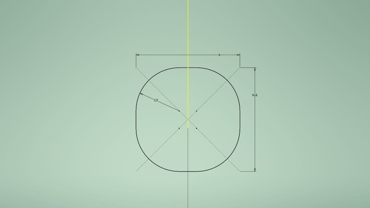
- Select the Two Point Center Rectangle command in the Create panel of the Sketch tab. This creates a rectangle, positioning its center.
- Position its center at the point corresponding to the 30-mm arc that we’ve just inserted in the sketch by the Project Geometry command.
- Dimension all the sides with a length of 6 mm.
- Select the Fillet command in the Create panel of the Sketch tab.
- Round the four corners with a 2.5-mm fillet. The cross-section can be seen in the image above.
Step 10: Sweep the Handle
Now that we have the path and the handle’s cross section, it’s possible to use the Sweep command to effectively build the model of the handle. Before we do the Sweep, though, you’ll want to make the mug’s body visible again, so you’ll be able to see both bodies.
To execute the Sweep, we’ll have to define the Path and the Profile (i.e. the cross section sketch just created), as well as configure a few other noteworthy settings classified as Behavior and Output settings in the Sweep Property Panel. With the Behavior settings, it’s possible to change the orientation of the sketch along the path, taper, and twist angle. They include the following:
- Follow Path: The sketches will rotate to follow the path slope, perpendicular to it at each point.
- Fixed: The sketches along the path will remain always parallel to the original sketch.
- Guide: This case requires two paths, so the sketch will follow them as rails.
Output settings allow you to choose the Boolean output of the solid – that is, how the solid swept will be compared with a previously created body. The options include the following:
- Join: Both bodies will be added to form a single one.
- Cut: This new body will subtract the previous body.
- Intersect: Only the intersection between the two bodies will remain.
- New solid: Creates a new solid.
With all of that in mind, here’s how to do the Sweep:
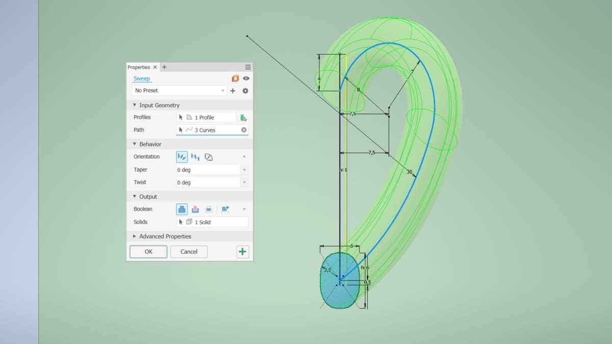
- Select the Sweep command in the Create panel of the 3D Model tab. The Sweep Property Panel will open.
- Select the Profile input box, then select the handle’s cross-sectional sketch.
- Select the Path input box, then select the path’s sketch.
- Under Behavior, choose the option Follow Path, so it will be perpendicular to the path curvature at each point.
- Keep the taper and twist angles set to 0 degrees.
- Under Output, select the Join icon for Boolean.
- Click Ok.
Step 11: Finalize the 3D Model
Since our mug model is now finished, we can fill it up with a beverage. To do this, we’ll work with surfaces in Inventor.
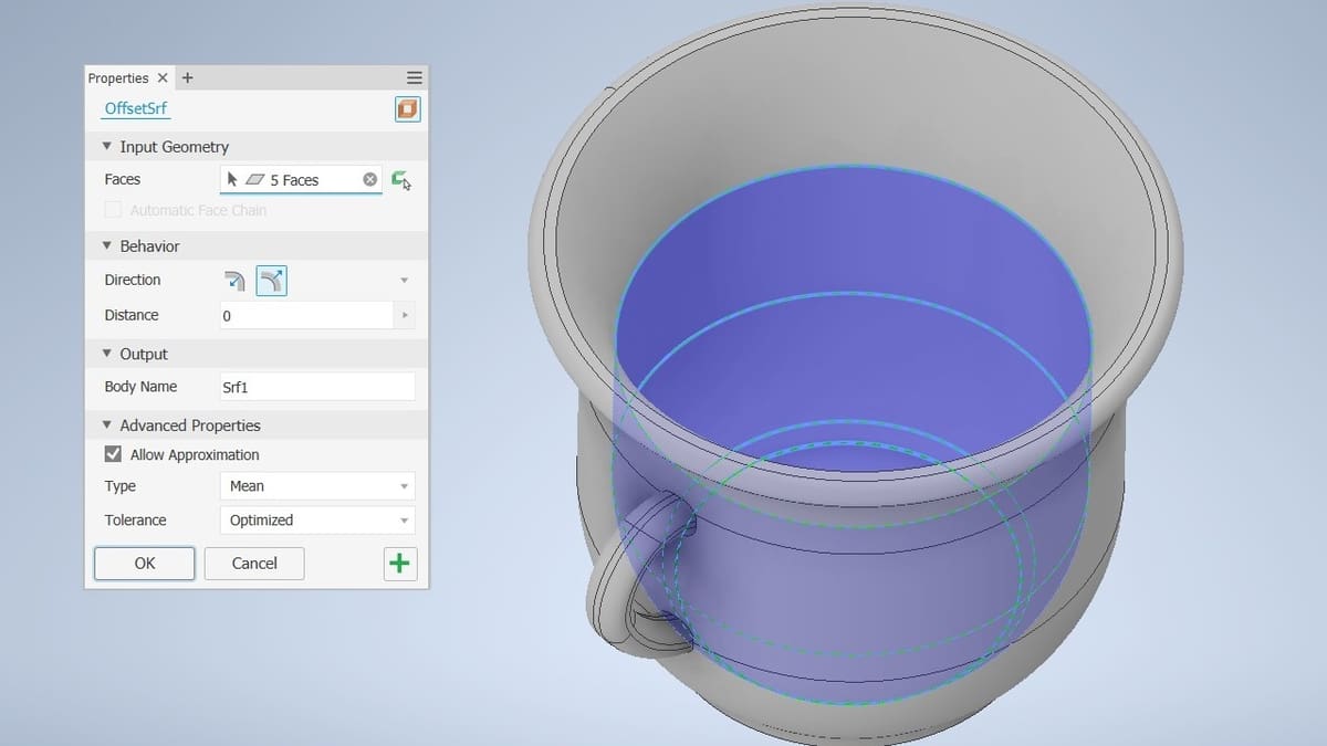
- Select the Thicken/Offset command in the Modify panel of the 3D Model tab. Liquids take the shape of their container, and by applying this command, we’ll be able to create surfaces from the inner faces of the mug model.
- When the Thicken/Offset Property Panel opens, click on the small orange button in the upper-right corner (Surface mode is ON).
- Select all the inner faces of the mug until the last revolution boundary. It should be five faces in total.
- In Behavior configurations, set the Distance to 0 (zero).
The image above shows the Thicken/Offset Property Panel configurations and the selections to make in this window.
To close the beverage surface, we’ll use the Patch command, which creates a surface delimited by some closed boundary. In the case of the mug, it will be chosen as the last revolution boundary of the body.
- Select the Patch command in the Surface panel of the 3D Model tab.
- When the Boundary Patch toolbar opens, click on the last revolving edge of the mug. This will be the surface of the beverage inside the mug.
- Click Apply.
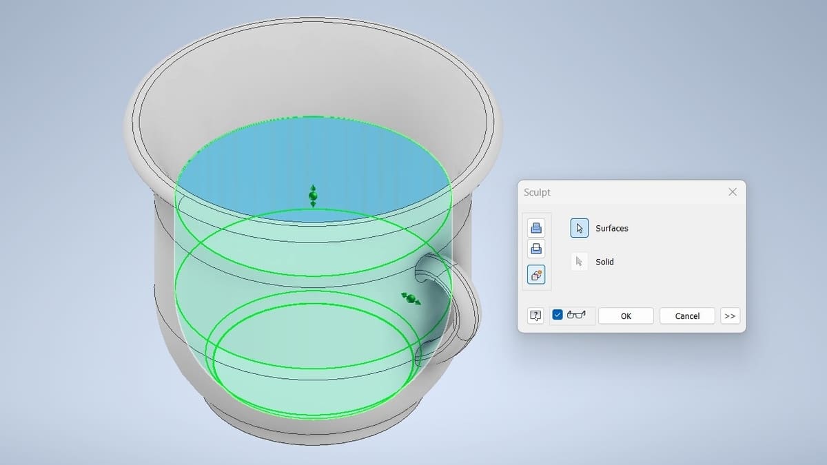
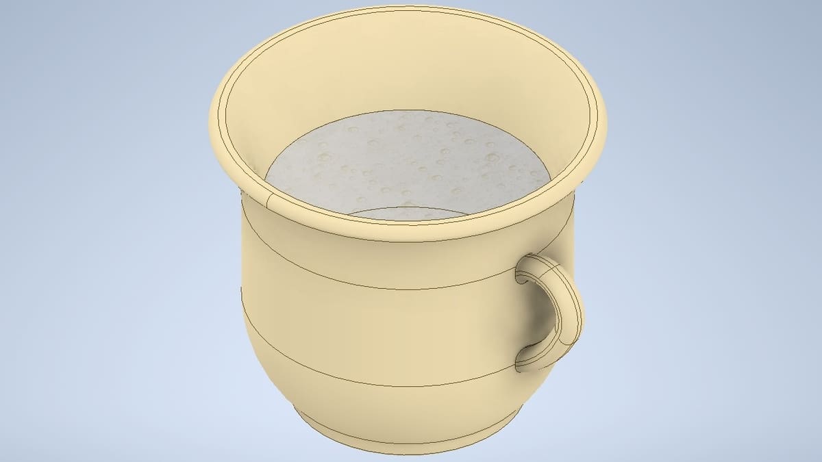
We now have a closed volume delimited by surfaces. If you turn off the mug’s body visibility, you can see it clearly in a transparent scale of orange. However, what we need is to turn this volume into real material. To do this, we’re going to use the Sculpt command, which adds material between surfaces:
- Select the Sculpt command in the Surface panel of the 3D Model tab.
- When the Sculpt toolbar opens, select from the Model Browser the patch and the surfaces created with the Thicken/Offset command.
- Similar to the Sweep Property Panel, you can choose the Boolean outputs of joining (Add button), removing (Remove button), or creating a new body (New Solid button). Let’s choose the New Solid output. A preview of the material addition will appear in green, as the image above shows.
- Go ahead and click Ok.

With this last step, the mug model is now complete, as shown in the image above. It’s composed of two bodies: the mug with a handle and the beverage. Considering the final result, this model is rather complicated. This is why it’s important to always analyze the object, then split the geometry in the main body and details, as well as to identify the orthogonal views of an object and start with a sketch. With Inventor and other parametric software, the preparation step is the most important for the success of your modeling.
Part III: Rendering
Although the mug model is complete, some other steps can be applied to take it to the next level. While they’re beyond the scope of this tutorial, we’ll briefly touch on the basics.
Materials & Rendering
Materials can be applied to a model to make it resemble the real object and make the simulation more precise. The easiest way to apply materials is with the Tools panel at the top of the Application Window. There are two boxes: one for the assigned Material and the other for the Appearance.
The final step for a model’s appearance is rendering, which involves manipulating the visualization of the design to make it resemble a real object or to build artistic images with the model. This can be accessed from the Environments ribbon tab, with the command Inventor Studio. Local lights and camera orientation can be manipulated, as well as the number of iterations to get the clearest image.
Step 12: Add Materials & Render the Model
To apply materials to our mug example, follow these steps:
- Click on the Material button in the Quick Access toolbar and search for “Porcelain”. The “Porcelain, Ivory” or “Porcelain, Linen” can be selected.
- From the Model Browser, open the folder Solid Bodies, then select the body related to the mug.
- Override its appearance to “Beige” by looking for it in the box next to the Material box in the Tools ribbon.
- From the Model Browser, open the folder Solid Bodies and select the body related to the beverage.
- Override its appearance to “Water Bubbles” by looking for it in the box next to the Material box in the Tools ribbon.
The rendering process can be applied with a first preparation in the View ribbon tab, as follows:
- Enter the View ribbon tab.
- In the Appearance panel, choose the Visual Style from among the Realistic and Shaded visualizations, which offer the most realistic rendering.
- You can change the way the model is seen in the Graphics Display and the rendering by changing the appearance of shadows (in the Shadows drop-down menu), reflections (in the Reflections drop-down menu), and the environment lights (in the Lighting Style drop-down menu). Also, it’s possible to change the projection type into orthographic, perspective, or perspective with ortho faces in the projection drop-down menu.
After these basic appearance configurations, let’s render the model using Inventor Studio:
- Enter the Environments ribbon tab, then click on Inventor Studio in the Begin panel. There are advanced parameters here for light positions, shadows, and camera. For your first time rendering, let’s skip these configurations and follow the next step.
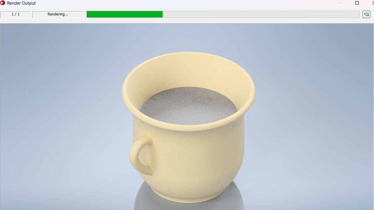
- Click on the Render Image button on the Render panel. From here, the Render Output window will open, showing the scene of the model being rendered in real-time and a green progress bar on the top.
- When the green bar indicates the iteration is finished, you can click the teapot icon in the upper-right corner to render again, increasing the render iteration steps. The more iteration steps, the clearer the image, but the longer the render process will be.
- When the image achieves your desired appearance, click the save button, saving your render scene as an image.
Tip
As we said above, increasing the iteration steps results in a clearer image at the expense of render time. Eventually, you’ll realize that it will reach an optimal result and that more iterations will add only a minimal enhancement. If you want to increase the image refinement from that point, you must return to step 1 and change the advanced parameters of lights and cameras.
Further Steps
If you want to take your model to the next level, there are a couple of additional steps you can complete in Inventor.
Assembly
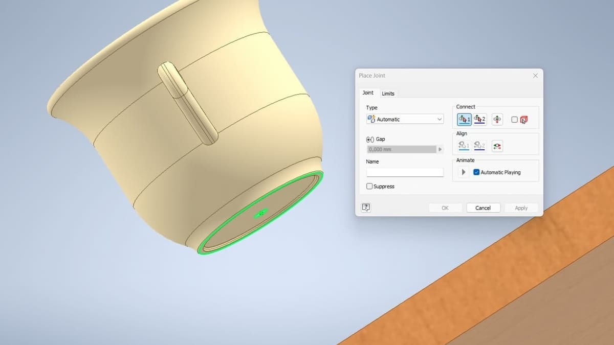
In some cases, it’s necessary to assemble parts saved in different Inventor files. This can be done with the Assembly tools. The Assemble environment cannot be accessed from the Part environment, so you’ll need to create a new Assembly document.
It’s possible to join parts and apply constraints to your model from here. Mechanical parts, such as bolts and nuts, are standardized, so there’s a Content Center where you can import commonly used types into your assembly to ensure everything fits together properly.
Simulation
Autodesk Inventor can be used directly in engineering simulations, as it’s a practical alternative for professionals who often have to deal with dedicated software. In the Environments panel of a Part drawing, there is a Stress Analysis command. Considering the principles of finite element analysis, a mathematical approach for calculating the internal stresses, and the strains of mechanical parts, the Analysis environment provides helpful tools for checking the strength of the model right where it can be modified directly.
License: The text of "Autodesk Inventor Tutorial for Beginners: 12 Steps to Success" by All3DP is licensed under a Creative Commons Attribution 4.0 International License.